Title here
Summary here
This article follows Introduction to Power Analysis with the ChipWhisperer, in which we captured power traces and visually identified the ten rounds of AES.
We now know that the microcontroller’s power consumption depends on the data it is processing. The next step is to turn that observation into an attack: recovering the encryption key from the traces alone, without access to the code or the hardware. That is the purpose of DPA (Differential Power Analysis), introduced in 1999 by Paul Kocher, Joshua Jaffe, and Benjamin Jun. The principle: from a hypothesis on one key byte, predict an intermediate bit of the cipher, use it to split the traces into two groups, then compute the difference of the means. If the hypothesis is correct, a spike appears; otherwise, the difference stays flat.
That is the mechanism we will detail and implement in the following sections.
The DPA algorithm (simplified here for simulation purposes) rests on a simple idea: the power consumption measured at any given instant mixes two things. One part depends on the data the chip is currently processing, which is the information we are after. The other part is noise, meaning everything that pollutes the measurement without relation to that data (electronic noise, electromagnetic interference, activity from the rest of the circuit). The entire attack consists in isolating the first by neutralising the second.
To do this, we rely on a property of noise: it is random and centred, meaning it pulls the consumption sometimes up, sometimes down, with no preferred direction. On a single trace, it can be stronger than the signal and completely mask the information. But if we sum many traces and average them, these random deviations compensate each other and eventually disappear. The signal, on the other hand, does not cancel out: since it always depends on the same data, it accumulates. Averaging therefore acts as a filter that erases randomness and lets the useful part emerge.
Illustrated example in Python:
import random
random.seed(0)

# leakage model: consumption depends on the bit value
def consumption(bit):
    if bit == 1:
        return 1 + random.gauss(0, 1)   # processing a 1 costs slightly more
    if bit == 0:
        return 0 + random.gauss(0, 1)   # processing a 0 costs slightly less

bits   = []
consos = []
for _ in range(1000):
    bit = random.randint(0, 1)
    bits.append(bit)
    consos.append(consumption(bit))

def difference(hypothesis):
    group1 = [consos[i] for i in range(1000) if hypothesis[i] == 1]
    group0 = [consos[i] for i in range(1000) if hypothesis[i] == 0]
    return sum(group1)/len(group1) - sum(group0)/len(group0)

random_hyp = [random.randint(0, 1) for _ in range(1000)]

print("Correct hypothesis  :", round(difference(bits), 3))
# 1.01
print("Wrong hypothesis    :", round(difference(random_hyp), 3))
# -0.074
What remains is to use this useful part to recover the key. The idea is to make a guess about the data being processed, then sort the traces into two groups based on that guess: on one side those where we assume a bit at 1, on the other those where we assume a 0. We compute the mean consumption of each group and look at the gap between them. If the guess was right, the two groups correspond to genuinely different consumptions and the gap is clear: that is the spike. If it was wrong, the split is random, the two groups look alike, and the gap collapses toward zero. All that remains is to try all possible guesses: the one that produces the spike reveals the correct value, and therefore the key.
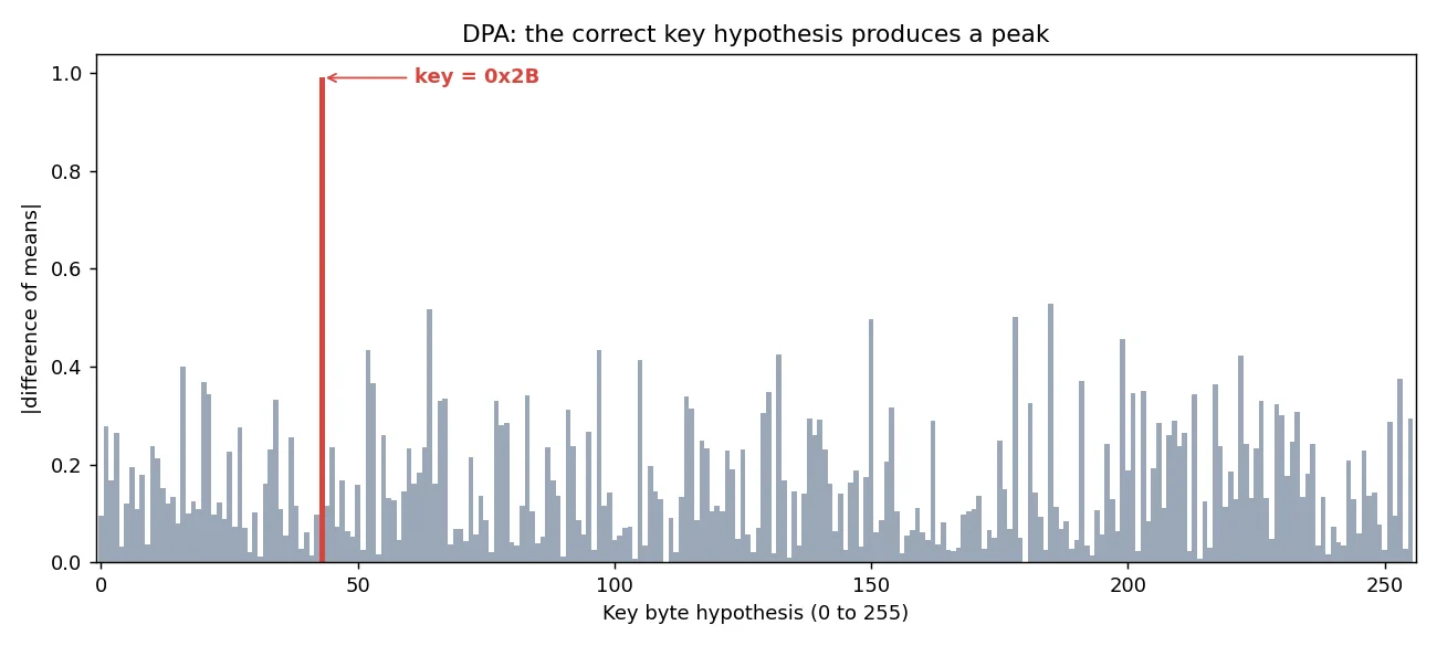
The AES algorithm breaks each round into four operations (AddRoundKey, SubBytes, ShiftRows, and MixColumns), all linear except the S-box (SubBytes). A linear operation means a change in the input has a predictable effect on the output. With the S-box, which is non-linear, two neighbouring hypotheses produce completely different predictions.
There is no need to target multiple bytes at once: we keep the same output byte and the same bit. Since the plaintexts vary, that bit takes the value 0 or 1 depending on the trace, which is enough to fill both groups of the partition.
Illustration example in Python:
import random
import numpy as np
random.seed(0)

# AES S-box
sbox = np.array([
    0x63,0x7c,0x77,0x7b,0xf2,0x6b,0x6f,0xc5,0x30,0x01,0x67,0x2b,0xfe,0xd7,0xab,0x76,
    0xca,0x82,0xc9,0x7d,0xfa,0x59,0x47,0xf0,0xad,0xd4,0xa2,0xaf,0x9c,0xa4,0x72,0xc0,
    0xb7,0xfd,0x93,0x26,0x36,0x3f,0xf7,0xcc,0x34,0xa5,0xe5,0xf1,0x71,0xd8,0x31,0x15,
    0x04,0xc7,0x23,0xc3,0x18,0x96,0x05,0x9a,0x07,0x12,0x80,0xe2,0xeb,0x27,0xb2,0x75,
    0x09,0x83,0x2c,0x1a,0x1b,0x6e,0x5a,0xa0,0x52,0x3b,0xd6,0xb3,0x29,0xe3,0x2f,0x84,
    0x53,0xd1,0x00,0xed,0x20,0xfc,0xb1,0x5b,0x6a,0xcb,0xbe,0x39,0x4a,0x4c,0x58,0xcf,
    0xd0,0xef,0xaa,0xfb,0x43,0x4d,0x33,0x85,0x45,0xf9,0x02,0x7f,0x50,0x3c,0x9f,0xa8,
    0x51,0xa3,0x40,0x8f,0x92,0x9d,0x38,0xf5,0xbc,0xb6,0xda,0x21,0x10,0xff,0xf3,0xd2,
    0xcd,0x0c,0x13,0xec,0x5f,0x97,0x44,0x17,0xc4,0xa7,0x7e,0x3d,0x64,0x5d,0x19,0x73,
    0x60,0x81,0x4f,0xdc,0x22,0x2a,0x90,0x88,0x46,0xee,0xb8,0x14,0xde,0x5e,0x0b,0xdb,
    0xe0,0x32,0x3a,0x0a,0x49,0x06,0x24,0x5c,0xc2,0xd3,0xac,0x62,0x91,0x95,0xe4,0x79,
    0xe7,0xc8,0x37,0x6d,0x8d,0xd5,0x4e,0xa9,0x6c,0x56,0xf4,0xea,0x65,0x7a,0xae,0x08,
    0xba,0x78,0x25,0x2e,0x1c,0xa6,0xb4,0xc6,0xe8,0xdd,0x74,0x1f,0x4b,0xbd,0x8b,0x8a,
    0x70,0x3e,0xb5,0x66,0x48,0x03,0xf6,0x0e,0x61,0x35,0x57,0xb9,0x86,0xc1,0x1d,0x9e,
    0xe1,0xf8,0x98,0x11,0x69,0xd9,0x8e,0x94,0x9b,0x1e,0x87,0xe9,0xce,0x55,0x28,0xdf,
    0x8c,0xa1,0x89,0x0d,0xbf,0xe6,0x42,0x68,0x41,0x99,0x2d,0x0f,0xb0,0x54,0xbb,0x16], dtype=np.uint8)

def hamming(x):
    return bin(x).count("1")

KEY = 0x2B          # the key byte to recover (unknown to the attacker)
N = 4000

# --- Device simulation ---
# the attacker knows the plaintexts; power consumption leaks the S-box output
plaintexts = [random.randint(0, 255) for _ in range(N)]
power = [hamming(sbox[p ^ KEY]) + random.gauss(0, 1) for p in plaintexts]

# --- Attack: try all 256 possible key bytes ---
def difference(guess):
    # for each trace, PREDICT one bit of the S-box output under hypothesis 'guess'
    predicted_bit = [(sbox[plaintexts[i] ^ guess] & 1) for i in range(N)]
    group1 = [power[i] for i in range(N) if predicted_bit[i] == 1]
    group0 = [power[i] for i in range(N) if predicted_bit[i] == 0]
    return sum(group1)/len(group1) - sum(group0)/len(group0)

diffs = [abs(difference(g)) for g in range(256)]
found = max(range(256), key=lambda g: diffs[g])

print(f"Actual key    : 0x{KEY:02X}")
print(f"Recovered key : 0x{found:02X}")Using the setup from the previous exercise, the notebook is split into two cells: first the trace capture, then the attack.
The two cells are intentionally separate. Capture takes a long time; once the traces are in memory, the attack can be re-run on its own while adjusting parameters, without going back through the hardware.
Cell 1: trace capture
import chipwhisperer as cw
import chipwhisperer.analyzer as cwa
import numpy as np

N = 4000
ktp = cw.ktp.Basic()

project = cw.create_project("sca101_dpa", overwrite=True)
for i in range(N):
    key, text = ktp.next()
    trace = cw.capture_trace(scope, target, text, key)
    if trace is not None:
        project.traces.append(trace)
    if i % 100 == 0:
        print(f"{i}/{N}")
Cell 2: DPA attack on all 16 bytes
Only M = 2500 traces out of the 4000 captured are used. M is a test parameter: by varying it without recapturing, we determine empirically how many traces are needed to recover the key. After several runs, below 2000 traces errors appear on some bytes; above that threshold, the attack converges consistently.
sbox = np.array([
    0x63,0x7c,0x77,0x7b,0xf2,0x6b,0x6f,0xc5,0x30,0x01,0x67,0x2b,0xfe,0xd7,0xab,0x76,
    0xca,0x82,0xc9,0x7d,0xfa,0x59,0x47,0xf0,0xad,0xd4,0xa2,0xaf,0x9c,0xa4,0x72,0xc0,
    0xb7,0xfd,0x93,0x26,0x36,0x3f,0xf7,0xcc,0x34,0xa5,0xe5,0xf1,0x71,0xd8,0x31,0x15,
    0x04,0xc7,0x23,0xc3,0x18,0x96,0x05,0x9a,0x07,0x12,0x80,0xe2,0xeb,0x27,0xb2,0x75,
    0x09,0x83,0x2c,0x1a,0x1b,0x6e,0x5a,0xa0,0x52,0x3b,0xd6,0xb3,0x29,0xe3,0x2f,0x84,
    0x53,0xd1,0x00,0xed,0x20,0xfc,0xb1,0x5b,0x6a,0xcb,0xbe,0x39,0x4a,0x4c,0x58,0xcf,
    0xd0,0xef,0xaa,0xfb,0x43,0x4d,0x33,0x85,0x45,0xf9,0x02,0x7f,0x50,0x3c,0x9f,0xa8,
    0x51,0xa3,0x40,0x8f,0x92,0x9d,0x38,0xf5,0xbc,0xb6,0xda,0x21,0x10,0xff,0xf3,0xd2,
    0xcd,0x0c,0x13,0xec,0x5f,0x97,0x44,0x17,0xc4,0xa7,0x7e,0x3d,0x64,0x5d,0x19,0x73,
    0x60,0x81,0x4f,0xdc,0x22,0x2a,0x90,0x88,0x46,0xee,0xb8,0x14,0xde,0x5e,0x0b,0xdb,
    0xe0,0x32,0x3a,0x0a,0x49,0x06,0x24,0x5c,0xc2,0xd3,0xac,0x62,0x91,0x95,0xe4,0x79,
    0xe7,0xc8,0x37,0x6d,0x8d,0xd5,0x4e,0xa9,0x6c,0x56,0xf4,0xea,0x65,0x7a,0xae,0x08,
    0xba,0x78,0x25,0x2e,0x1c,0xa6,0xb4,0xc6,0xe8,0xdd,0x74,0x1f,0x4b,0xbd,0x8b,0x8a,
    0x70,0x3e,0xb5,0x66,0x48,0x03,0xf6,0x0e,0x61,0x35,0x57,0xb9,0x86,0xc1,0x1d,0x9e,
    0xe1,0xf8,0x98,0x11,0x69,0xd9,0x8e,0x94,0x9b,0x1e,0x87,0xe9,0xce,0x55,0x28,0xdf,
    0x8c,0xa1,0x89,0x0d,0xbf,0xe6,0x42,0x68,0x41,0x99,0x2d,0x0f,0xb0,0x54,0xbb,0x16], dtype=np.uint8)

textins  = np.array([t.textin for t in project.traces], dtype=np.uint8)
traces   = np.array([t.wave   for t in project.traces])

M = 2500
textins = textins[:M]
traces  = traces[:M]

real_key = np.array(project.traces[0].key, dtype=np.uint8)

def diff(guess, byte=0):
    inter = sbox[textins[:, byte] ^ guess]
    bit = inter & 1
    mean1 = traces[bit == 1].mean(axis=0)
    mean0 = traces[bit == 0].mean(axis=0)
    return mean1 - mean0

def attack_byte(byte=0):
    peaks = []
    for guess in range(256):
        d = diff(guess, byte)
        peaks.append(np.max(np.abs(d)))
    return int(np.argmax(peaks))

key = []
for b in range(16):
    guess = attack_byte(b)
    key.append(guess)
    ok = "OK" if guess == real_key[b] else "X"
    print(f"byte {b:2d} : guess = 0x{guess:02X}   real = 0x{real_key[b]:02X}   {ok}")
KeyboardInterrupt Traceback (most recent call last)
Cell In[30], line 44
42 key = []
43 for b in range(16):
---> 44 guess = attack_byte(b)
Cell In[30], line 38, in attack_byte(byte)
36 peaks = []
37 for guess in range(256):
---> 38 d = diff(guess, byte)
Cell In[30], line 32, in diff(guess, byte)
29 inter = sbox[textins[:, byte] ^ guess]
30 bit = inter & 1
31 mean1 = traces[bit == 1].mean(axis=0)
---> 32 mean0 = traces[bit == 0].mean(axis=0)In practice this version is too slow: for each byte it iterates over 256 hypotheses and recomputes two means over 2500 traces each time, for 16 bytes total, that is 16 x 256 = 4096 passes over the full dataset. The Python loop cannot keep up.
The solution is to vectorise: rather than processing one hypothesis at a time, all 256 are computed in a single matrix operation. NumPy no longer runs Python per iteration but a single optimised matrix product.
def attack_byte_fast(byte=0):
    pt = textins[:, byte]                                               # (M,)
    guesses = np.arange(256, dtype=np.uint8)
    inter = sbox[np.bitwise_xor(pt[None, :], guesses[:, None])]        # (256, M)
    bits = (inter & 1).astype(np.float32)                              # (256, M)

    counts1 = bits.sum(axis=1, keepdims=True)                          # (256, 1)
    counts0 = M - counts1

    mean1 = (bits @ traces) / counts1                                  # (256, T)
    mean0 = ((1 - bits) @ traces) / counts0

    peaks = np.abs(mean1 - mean0).max(axis=1)                          # (256,)
    return int(np.argmax(peaks))

key = []
for b in range(16):
    guess = attack_byte_fast(b)
    key.append(guess)
    ok = "OK" if guess == real_key[b] else "X"
    print(f"byte {b:2d} : guess = 0x{guess:02X}   real = 0x{real_key[b]:02X}   {ok}")
byte 0 : guess = 0x2B real = 0x2B OK
byte 1 : guess = 0x7E real = 0x7E OK
byte 2 : guess = 0x15 real = 0x15 OK
byte 3 : guess = 0x16 real = 0x16 OK
byte 4 : guess = 0x28 real = 0x28 OK
byte 5 : guess = 0xAE real = 0xAE OK
byte 6 : guess = 0xD2 real = 0xD2 OK
byte 7 : guess = 0xA6 real = 0xA6 OK
byte 8 : guess = 0xAB real = 0xAB OK
byte 9 : guess = 0xF7 real = 0xF7 OK
byte 10 : guess = 0x15 real = 0x15 OK
byte 11 : guess = 0x88 real = 0x88 OK
byte 12 : guess = 0x09 real = 0x09 OK
byte 13 : guess = 0xCF real = 0xCF OK
byte 14 : guess = 0x4F real = 0x4F OK
byte 15 : guess = 0x3C real = 0x3C OKAll 16 bytes are recovered correctly. The full key 2b7e151628aed2a6abf7158809cf4f3c matches the AES key used by the firmware.
The implementation presented here is not the most optimised: NumPy vectorisation helps, but DPA remains intrinsically expensive. For each byte, a difference of means is computed over the full trace set for all 256 hypotheses, repeated 16 times. On real hardware with thousands of traces, that cost is felt.
That cost is however the price of pedagogy: DPA is the conceptually simplest side-channel attack. It lays the groundwork without requiring any leakage model beyond the S-box output bit. Understanding why it works is understanding why all subsequent statistical attacks work.
The next article introduces CPA (Correlation Power Analysis), which replaces the difference of means with a Pearson correlation and a Hamming weight leakage model. In practice, CPA converges with far fewer traces and is significantly faster to compute.